Overview

Being able to load and manipulate data is the first step towards rendering a scene. simple-3dviz implements various Renderables such as meshes, point clouds, lines e.t.c that can be used for configuring different types of input.

Creating Meshes

simple-3dviz allows you to configure a Mesh from a file, a set of vertices and normals, a voxel grid or a set of geometric primitives, which we model using superquadric surfaces.

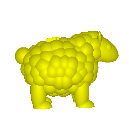
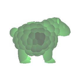
Loading meshes from files can be easily done using the Mesh.from_file() method. Note that the supported mesh file formats are .obj, .off, .stl and .ply.

>>> from simple_3dviz import Mesh
>>> m = Mesh.from_file("models/sheep.stl")

# It is possible to load a mesh with any color you like
>>> m = Mesh.from_file("models/sheep.stl", color=(1, 1, 0))
# And with transparency
>>> m = Mesh.from_file("models/sheep.stl", color=(0.3, 1, 0.3, 0.6))

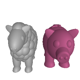
# It is also possible to manipulate the position of a mesh in a scene by
# properly adjusting its offset
>>> m = Mesh.from_file("models/sheep.stl", color=(0.8, 0.8, 0.8))
>>> m2 = Mesh.from_file("models/pig.stl", color=(0.8, 0.38, 0.58))
>>> m2.offset = (45, 0, 0)

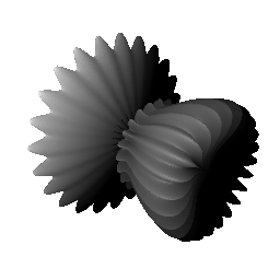
You can also create a Mesh from a set of 3D points using the Mesh.from_xyz() method, from a set of vertices and faces using the Mesh.from_faces() method or using a set of vertices and normals.

>>> from simple_3dviz import Mesh

# Let us visualize a spherical harmonic as a surface similar to
# https://docs.enthought.com/mayavi/mayavi/mlab.html
>>> import numpy as np
>>> dphi, dtheta = np.pi/250.0, np.pi/250.0
>>> [phi, theta] = np.mgrid[0:np.pi+dphi*1.5:dphi, 0:2*np.pi+dtheta*1.5:dtheta]
>>> m0 = 4; m1 = 3; m2 = 2; m3 = 3; m4 = 6; m5 = 2; m6 = 6; m7 = 4;
>>> r = np.sin(m0 * phi)**m1 + np.cos(m2 * phi)**m3
>>> r = r + np.sin(m4 * theta)**m5 + np.cos(m6 * theta)**m7
>>> x = r * np.sin(phi) * np.cos(theta)
>>> y = r * np.cos(phi)
>>> z = r * np.sin(phi) * np.sin(theta)

>>> m = Mesh.from_xyz(x, y, z)

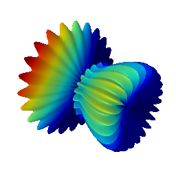
# It is also possible to load a mesh with a colormap
>>> import matplotlib.pyplot as plt
>>> m = Mesh.from_xyz(x, y, z, colormap=plt.cm.jet)

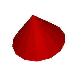
# We visualize a cone defined using vertices and faces, similar to
# https://docs.enthought.com/mayavi/mayavi/auto/mlab_helper_functions.html#points3d
>>> t = np.linspace(-np.pi, np.pi, 16)
>>> z = np.exp(1j * t)
>>> x = z.real.copy()
>>> y = z.imag.copy()
>>> z = np.zeros_like(x)
>>> 
>>> faces = [(0, i, i + 1) for i in range(1, 16)]
>>> x = np.r_[0, x]
>>> y = np.r_[0, y]
>>> z = np.r_[1, z]
>>> vertices = np.stack([x, y, z]).T
>>> colors = np.ones((len(points), 3))*[1.0, 0.0, 0.0]
>>> m = Mesh.from_faces(vertices, faces, colors=colors)

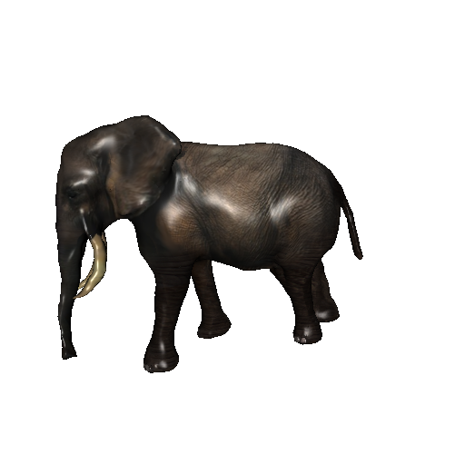
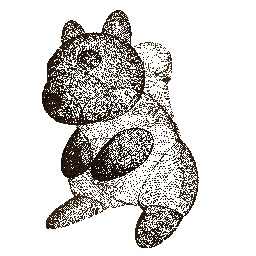
Creating Textured Meshes

simple-3dviz also supports rendering meshes with textures. To load a mesh with a texture/material you can use the TexturedMesh class similar to the way you would use Mesh.

>>> from simple_3dviz import TexturedMesh
>>> from simple_3dviz.behaviours.misc import LightToCamera
>>> from simple_3dviz.window import show

# The model together with its material files is downloaded for free from
# https://www.turbosquid.com/3d-models/african-elephant-obj-free/1126601
>>> m = TexturedMesh.from_file("path/to/elefante.obj")
>>> show(
...     m,
...     behaviours=[LightToCamera()],
...     camera_position=(8, 8, 8),
...     up_vector=(0, 1, 0)
... )

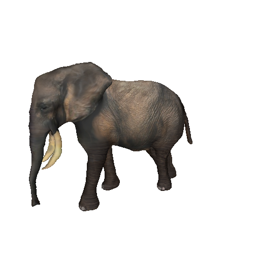
# You can also set the material after loading the model
>>> from simple_3dviz.renderables.textured_mesh import Material
>>> mtl = Material.with_texture_image(
...     "path/to/elefantefull.png",
...     ambient=(0.4, 0.4, 0.4),
...     diffuse=(0.4, 0.4, 0.4),
...     specular=(0.1, 0.1, 0.1),
...     Ns=2
... )
>>> m.material = mtl
>>> show(
...     m,
...     behaviours=[LightToCamera()],
...     camera_position=(8, 8, 8),
...     up_vector=(0, 1, 0)
... )

Note that is is also possible to render textured meshes with multiple materials. You can again load a textured mesh with multiple materials using the TexturedMesh class as we did previously. In the following example you can see how you can render a 3D mesh with multiple materials, render it from various view points and save the animation as a gif.

>>> from simple_3dviz.behaviours.io import SaveGif
>>> from simple_3dviz.behaviours.movements import CameraTrajectory
>>> from simple_3dviz.behaviours.trajectory import Circle
>>> from simple_3dviz.renderables import TexturedMesh
>>> from simple_3dviz.utils import render, save_frame

# The 3D model together with its material is from ShapeNet
>>> rr1 = TexturedMesh.from_file("/tmp/motorbikes/motorbike_1.obj")
# Transfer the mesh to the unit cube
>>> rr1.to_unit_cube()
# Scale and transfer the mesh within a unit cube
>>> render(
...    rr1,
...    [
...        CameraTrajectory(
...            Circle((0, 0, 0), (0.0, 0.60, 1.4), (0, -1, 0)),
...            speed=1/180
...        ),
...        SaveGif("/tmp/motorbike_1.gif")
...    ],
...    up_vector=(0, 1, 0),
...    size=(1200, 1200),
...    camera_position=(0.0, 0.60, 1.4),
...    light=(0,5,0)
... )

# The 3D model together with its material is from ShapeNet
>>> rr2 = TexturedMesh.from_file("/tmp/motorbikes/motorbike_2.obj")
# Render the scene and save the animation as a gif
>>> render(
...    rr2,
...    [
...        CameraTrajectory(
...            Circle((0, 0, 0), (0.0, 0.4, 1.0), (0, -1, 0)),
...            speed=1/180
...        ),
...        SaveGif("/tmp/motorbike_2.gif")
...    ],
...    180,
...    camera_position=(0.0, 0.4, 1.0),
...    light=(0,)*3,
...    background=(1,)*4,
...    up_vector=(0, 1, 0)
...)

# It is possible to turn off the culling of faces that are pointing away
# from the camera, which by default is set to true
>>> if hasattr(rr2, "renderables"):
...     for r in rr2.renderables:
...         r.cull_back_face = False
... else:
...     rr2.cull_back_face = False

# Render the scene and save the animation as a gif
>>> render(
...    rr2,
...    [
...        CameraTrajectory(
...            Circle((0, 0, 0), (0.0, 0.4, 1.0), (0, -1, 0)),
...            speed=1/180
...        ),
...        SaveGif("/tmp/motorbike_3.gif")
...    ],
...    180,
...    camera_position=(0.0, 0.4, 1.0),
...    light=(0,)*3,
...    background=(1,)*4,
...    up_vector=(0, 1, 0)
...)

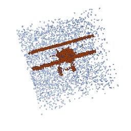
Creating Voxel Grids

It is possible to create a Mesh containing a voxel grid directly from an array of 3D values, where true values indicate the voxels to be filled using the Mesh.from_voxel_grid() method.

>>> from simple_3dviz import Mesh
>>> from simple_3dviz.window import show

# We create a NxNxN voxel grid with True values if the voxel is inside a heart
# object and False otherwise. We implement the Taubin's heart surface as
# described
# https://www.wolframalpha.com/input/?i=taubin%27s+heart+surface
>>> import numpy as np
>>> N = 64
>>> x = np.linspace(-1.3, 1.3, N)
>>> y = np.linspace(-1.3, 1.3, N)
>>> z = np.linspace(-1.3, 1.3, N)
>>> x, y, z = np.meshgrid(x, y, z)
>>> voxels = (2*x**2 + y**2 + z**2-1)**3 - (1/10) * x**2*z**3 - y**2*z**3 < 0
>>> m = Mesh.from_voxel_grid(voxels, colors=(0.8, 0, 0))
>>> show(m)

# It is also possible to visualize the voxel grid with boundaries by creating
# a Lines renderable object
>>> from simple_3dviz import Lines
>>> l = Lines.from_voxel_grid(voxels, colors=(0, 0, 0.), width=0.01)
>>> show([m, l])

Creating Point clouds

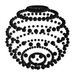
simple-3dviz also allows you to create and manipulate a point cloud directly from a numpy array using the Spherecloud renderable.

>>> from simple_3dviz import Spherecloud
>>> import numpy as np

>>> def fexp(x, p):
...     return np.sign(x)*(np.abs(x)**p)

# Define the parametric function of superquadric surfaces
>>> def sq_surface(a1, a2, a3, e1, e2, eta, omega):
...     x = a1 * fexp(np.cos(eta), e1) * fexp(np.cos(omega), e2)
...     y = a2 * fexp(np.cos(eta), e1) * fexp(np.sin(omega), e2)
...     z = a3 * fexp(np.sin(eta), e1)
...     return x, y, z

# Sample points on the surface of the supequadric
>>> eta = np.linspace(-np.pi/2, np.pi/2, 100, endpoint=True)
>>> omega = np.linspace(-np.pi, np.pi, 100, endpoint=True)
>>> eta, omega = np.meshgrid(eta, omega)
>>> x, y, z = sq_surface(a1=0.4, a2=0.4, a3=0.4, e1=1.0, e2=1.0, eta=eta, omega=omega)
>>> centers = np.stack([x, y, z]).reshape(3, -1).T
>>> s = Spherecloud(centers[::30])

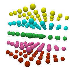
# It is possible to modify the color and the size of the rendered point cloud
# by properly setting the colors and sizes arguments.
>>> x = np.linspace(-0.5, 0.5, num=5)
>>> centers = np.array(np.meshgrid(x, x, x)).reshape(3, -1).T
>>> colors = np.ones((centers.shape[0], 4))
>>> colors[centers[:, 1] == -0.5] = [1, 1, 0, 1]
>>> colors[centers[:, 1] == -0.25] = [0, 1, 1, 1]
>>> colors[centers[:, 1] == 0] = [0.2, 0.8, 0.3, 1]
>>> colors[centers[:, 1] == 0.25] = [1.0, 0.41, 0.7, 1]
>>> colors[centers[:, 1] == 0.5] = [0.8, 0.2, 0, 1]
>>> sizes = np.ones(centers.shape[0])*0.05
>>> s = Spherecloud(centers, colors=colors, sizes=sizes)

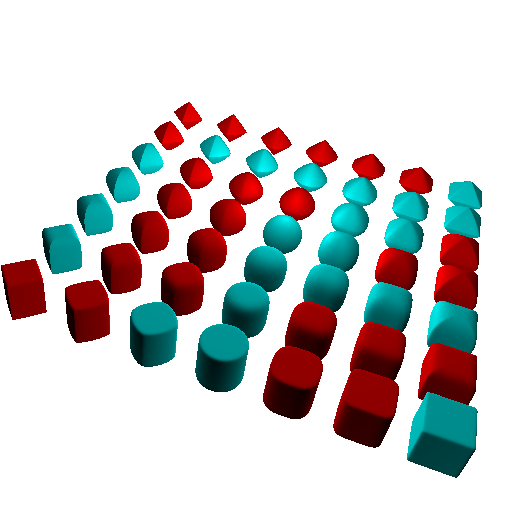
Creating Geometric Primitives

We use superquadric surfaces for modelling geometric primitives. Superquadrics are a parametric family of shapes that can represent various shapes using the same continuous space. They can be fully described with just 11 parameters, 2 for the shape, 3 for the size and 6 for the pose in the 3d space. With simple-3dviz, you can easily create a Mesh containing a set of primitives using the Mesh.from_superquadrics() function.

>>> import numpy as np
>>> from simple_3dviz import Mesh

# We will render various superquadrics with different shape parameters e1 and
# e2
>> N = 7

# SQs shapes
>>> e2 = np.linspace(0.1, 1.9, N, endpoint=True)
>>> e1 = np.linspace(0.1, 1.9, N, endpoint=True)
>>> epsilon_1, epsilon_2 = np.meshgrid(e1, e2)
>>> epsilon = np.stack([epsilon_1, epsilon_2]).reshape(2, -1).T

# SQs sizes
>>> alpha = np.ones((epsilons.shape[0], 3))
# SQs translations
>>> s = np.ceil(N*2.5 / 2)
>>> x = np.linspace(-s, s, N)
>>> y = np.linspace(-s, s, N)
>>> z = np.array([0])
>>> X, Y, Z = np.meshgrid(x, y, z)
>>> translation = np.stack([X, Y, Z]).reshape(3, -1).T

# SQs rotations
>>> rotation = np.eye(3)[np.newaxis] * np.ones((len(epsilons), 1, 1))

>>> colors = np.array([[1., 0, 0, 1],
...                    [0, 1, 1, 1]])[np.random.randint(0, 2, size=epsilons.shape[0])]

>>> m = Mesh.from_superquadrics(alpha, epsilon, translation, rotation, colors)

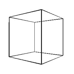
Creating Lines

simple-3dviz allows you to create lines directly from a numpy array that contains the line segments using the Lines object. Similar to the above, it is possible to adjust both the size and the color of each line segment.

>>> from simple_3dviz import Lines

# Create the line segments that yield a cube
>>> l = Lines([
            [-0.6, -0.6, -0.6], 
            [-0.6, -0.6,  0.6],
            [-0.6, -0.6,  0.6], 
            [-0.6,  0.6,  0.6],
            [-0.6,  0.6,  0.6], 
            [-0.6,  0.6, -0.6],
            [-0.6,  0.6, -0.6], 
            [-0.6, -0.6, -0.6],
            [ 0.6, -0.6, -0.6], 
            [ 0.6, -0.6,  0.6],
            [ 0.6, -0.6,  0.6], 
            [ 0.6,  0.6,  0.6],
            [ 0.6,  0.6,  0.6], 
            [ 0.6,  0.6, -0.6],
            [ 0.6,  0.6, -0.6], 
            [ 0.6, -0.6, -0.6],
            [ 0.6,  0.6,  0.6],
            [-0.6,  0.6,  0.6],
            [ 0.6,  0.6, -0.6],
            [-0.6,  0.6, -0.6],
            [ 0.6, -0.6,  0.6],
            [-0.6, -0.6,  0.6],
            [ 0.6, -0.6, -0.6],
            [-0.6, -0.6, -0.6],
        ], (0.1, 0.1, 0.1, 1.0), width=0.02)

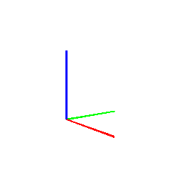
# Create axes
>>> l = Lines([
            [0.0, 0.0, 0.0],
            [0.6, 0.0, 0.0],
            [0.0, 0.0, 0.0],
            [0.0, 0.6, 0.0],
            [0.0, 0.0, 0.0],
            [0.0, 0.0, 0.6]
        ],
        colors = np.array([
            [1.0, 0.0, 0.0, 1.0],
            [1.0, 0.0, 0.0, 1.0],
            [0.0, 1.0, 0.0, 1.0],
            [0.0, 1.0, 0.0, 1.0],
            [0.0, 0.0, 1.0, 1.0],
            [0.0, 0.0, 1.0, 1.0]
        ]), width=0.02)